Using GeoKrige with rasterio

Intro

In numerous scenarios, users may already possess a mesh grid in a raster file format. To facilitate this scenario, the GeoKrige package incorporates a suitable transformer that simplifies the extraction of such mesh grids into an object structured exactly the same as the output of the numpy.meshgrid function.

Additionally, the built-in transformer streamlines the process of effortlessly generating new raster files based on a loaded raster file.

Load tutorial data

from geokrige.tutorials import data_df

data_df.info()
data_df.head(5)

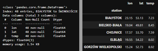
The loaded data represents mean air temperature values for 48 synoptic stations situated in Poland. The dataset spans from 1966 to 2020. It is stored as a DataFrame object, so it must be transformed to the numpy.ndarray object:

X = data_df[['lon', 'lat']].to_numpy()
y = data_df['temp'].to_numpy()

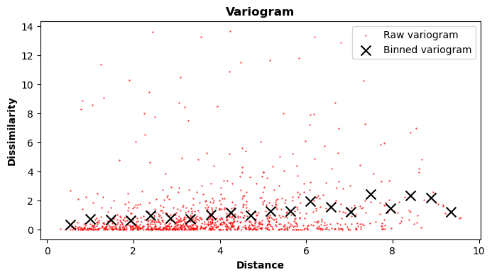
Initialize model & create a variogram

from geokrige.methods import OrdinaryKriging

kgn = OrdinaryKriging()
kgn.load(X, y)

In this tutorial, we will use the Ordinary Kriging Method. For further details regarding the distinctions between various Kriging Methods, please refer to this link.

kgn.variogram()

Fit function to the variogram

kgn.fit(model='exp')

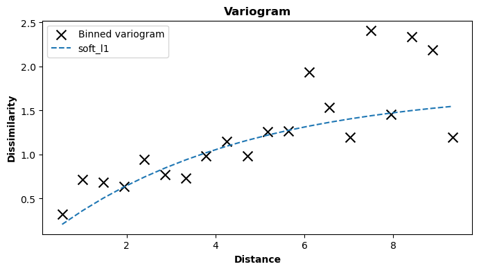
Here, the exponential variogram model is utilized, which effectively fits the data. For additional information regarding variogram models, please visit the Built-in Variogram Models section or refer to the Variogram - The Foundation of Any Kriging Method paragraph.

Prediction

The GeoKrige package offers the capability to transform raster objects into a mesh grid, which can then be passed to the predict method. For more information about mesh grids, please see this paragraph.

import rasterio
raster_file = 'europe_elevation.nc'
raster_file = rasterio.open(raster_file)
loaded_raster_Z = raster_file.read(1)  # europe's elevation as a mesh grid

Here, a raster file depicting Europe's elevation has been loaded. This data originates from the Copernicus DEM repository. Instructions for accessing and downloading the data can be found on the linked website. It is important to note that the data is subject to specific licensing terms and therefore is not bundled with the GeoKrige package. Alternatively, any other raster file covering the latitudes and longitudes of Poland can be used instead.

This is how the loaded data looks like:

Creating a mesh grid on the basis of the raster file

from geokrige.tools import TransformerRasterio

transformer = TransformerRasterio()
transformer.load(raster_file)

meshgrid = transformer.meshgrid()

In this manner, a mesh grid is generated and can subsequently be passed to the predict method. The resulting mesh grid possesses identical parameters (such as height, width, density, etc.) as the mesh grid stored within the loaded raster file. These similarities will become apparent later in this tutorial.

Using the created mesh grid to perform predictions

predicted_Z = kgn.predict(meshgrid)

Now, the predicted values for air temperature at specified points should precisely cover the same geographical area as the mesh grid stored within the loaded raster file. This alignment can be swiftly verified by comparing the shapes of both mesh grids:

print('Loaded mesh grid shape:', loaded_raster_Z.shape)
print('Predicted mesh grid shape:', predicted_Z.shape)

>>> Loaded mesh grid shape: (465, 705)
>>> Predicted mesh grid shape: (465, 705)

Visualizing results

import matplotlib.pyplot as plt

fig, ax = plt.subplots(1, 3, figsize=(18, 4))
X_lon, Y_lat = meshgrid

ax[0].set_title('Loaded elevation raster')
cbar = ax[0].pcolormesh(X_lon, Y_lat, loaded_raster_Z, cmap='Greys_r', vmin=-1000)
fig.colorbar(cbar, ax=ax[0])

ax[1].set_title('Predicted temperature values')
cbar = ax[1].pcolormesh(X_lon, Y_lat, predicted_Z, cmap='jet')
fig.colorbar(cbar, ax=ax[1])

ax[2].set_title('Overlaid elevation raster with predicted values')
ax[2].pcolormesh(X_lon, Y_lat, loaded_raster_Z, cmap='Greys_r', vmin=-1000)
cbar = ax[2].pcolormesh(X_lon, Y_lat, predicted_Z, cmap='jet', alpha=0.5)
fig.colorbar(cbar, ax=ax[2])

plt.show()

Since the data used to build the Kriging Model only covers Poland, the predictions outside Poland's borders are not accurate. However, the mesh grid created for predictions matches exactly the same area as the mesh grid stored in the loaded raster file, which is clearly visible in the plot above.

Saving mesh grids as a raster file

The TransformerRasterio object offers another handy feature, allowing users to save mesh grids into a newly created raster file (GeoTIFF file).

When creating a new raster file, the transformer will utilize parameters such as height, width, and shape from the loaded raster file. Consequently, the new raster file will be an exact replica of the loaded raster file, but with different layers (mesh grids) embedded within.

transformer.save(layers=[predicted_Z], path='predicted_temperature_values.tif')