Using GeoKrige with GeoPandas

Intro

The GeoKrige package primarily operates on numpy.ndarray objects. However, geospatial data is typically handled using the GeoPandas package. As a result, the GeoKrige package's load method is designed to accept GeoDataFrames.

Additionally, it includes a transformer that simplifies the conversion of POLYGONS into a mesh grid. This transformer can also generate a masking matrix for a mesh grid, enabling the selection of mesh grid values exclusively within POLYGONS boundaries.

Load tutorial data

from geokrige.tutorials import data_gdf

data_gdf.info()
data_gdf.head(5)

The loaded data represents mean air temperature values for 48 synoptic stations situated in Poland. The dataset spans from 1966 to 2020. It is stored as a GeoDataFrame object, with points represented in a geometry column. This geometry column is crucial for the GeoKrige package, as it will be utilized to calculate distances between points with known values.

data_gdf.geometry.head()

It is essential to note that the geometry column must exclusively contain points of type POINT when a GeoDataFrame object is passed to the load method.

Initialize model & create a variogram

from geokrige.methods import SimpleKriging

kgn = SimpleKriging()
kgn.load(data_gdf, y='temp')

In this tutorial, we will use the Simple Kriging Method. For further details regarding the distinctions between various Kriging Methods, please refer to this link.

When passing a GeoDataFrame object to the load method, the y parameter must specify the column name where the known values are stored. Spatial distances will be calculated based on the geometry column.

kgn.variogram()

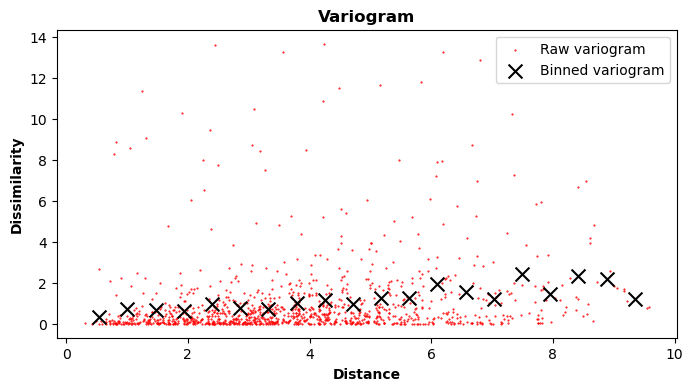
Fit function to the variogram

kgn.fit(model='exp')

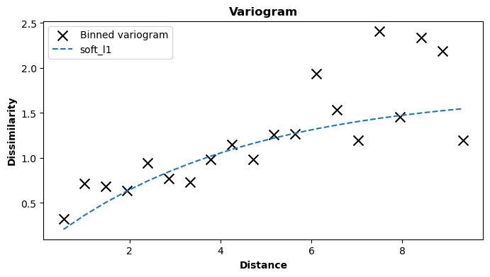
Here, the exponential variogram model is utilized, which effectively fits the data. For additional information regarding variogram models, please visit the Built-in Variogram Models section or refer to the Variogram - The Foundation of Any Kriging Method paragraph.

Prediction

The GeoKrige package offers the capability to transform POLYGONS stored within a GeoDataFrame object into a mesh grid, which can then be passed to the predict method. This process enables the creation of an interpolation map with ease. For more information about mesh grids, please see this paragraph.

import geopandas as gpd
shp_file = 'wojewodztwa.shp'
prediction_gdf = gpd.read_file(shp_file).to_crs(crs='EPSG:4326')

The shapefile containing Polish voivodeships can be downloaded from the www.gis-support.pl website. You can directly access the file by clicking here, or you can download the file from the website by clicking Województwa on the linked page.

After downloading the file, you need to extract its contents into a specific directory on your system. Once extracted, you can load the file with a .shp extension into a GeoDataFrame object.

Creating a mesh grid on the basis of a GeoDataFrame object & POLYGONS

from geokrige.tools import TransformerGDF

transformer = TransformerGDF()
transformer.load(prediction_gdf)

meshgrid = transformer.meshgrid(density=0.3)
mask = transformer.mask()

In this manner, a mesh grid is generated and can subsequently be passed to the predict method. Setting the density parameter to 0.3 implies that the resulting mesh grid will be less dense than by default. This difference will become evident later in the tutorial.

Using the created mesh grid to perform predictions

Z = kgn.predict(meshgrid)

The predict method will yield another matrix with the same shape as the matrices within the created mesh grid. Combining this returned matrix with the matrices in the meshgrid variable enables the straightforward creation of an interpolation map.

Visualizing results - with & without the mask

import matplotlib.pyplot as plt

fig, ax = plt.subplots()

data_gdf.plot(color='grey', zorder=6, ax=ax)  # known points
prediction_gdf.plot(facecolor='none', edgecolor='black', linewidth=1, zorder=5, ax=ax)  # borders

X_lon, Y_lat = meshgrid
cbar = ax.pcolormesh(X_lon, Y_lat, Z, cmap='jet', vmin=6, vmax=9)
fig.colorbar(cbar)

ax.set_title('Interpolation map without the mask')
plt.show()

fig, ax = plt.subplots()

data_gdf.plot(color='grey', zorder=6, ax=ax)  # known points
prediction_gdf.plot(facecolor='none', edgecolor='black', linewidth=1, zorder=5, ax=ax)  # borders

X_lon, Y_lat = meshgrid
Z[~mask] = None  # masking pixels out of boundaries
cbar = ax.pcolormesh(X_lon, Y_lat, Z, cmap='jet', vmin=6, vmax=9)
fig.colorbar(cbar)

ax.set_title('Interpolation map with the mask')
plt.show()

In this context, the previously created mask is used to conceal pixels that fall outside the POLYGONS delineated by the shapefile.

Utilizing the mask method yields a boolean matrix. A True value signifies that a given point resides within the boundaries of the POLYGONS.

Consequently, the masking matrix is inverted, as None values are assigned to points outside the POLYGONS. This signifies to the matplotlib package that the respective pixels should not be filled.

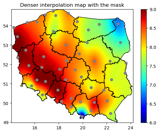
Creating a denser mesh grid

As mentioned earlier, the density of a mesh grid can be adjusted according to user preference. In previous instances, the mesh grid created might have been too sparse for some users. To address this, the density parameter can be utilized (it is set to 1 by default).

It is important to note that this parameter must be a positive float. Therefore, if the default grid density (1) is insufficient, it can be increased to 2, 3, and so forth. However, it is essential to be aware that denser mesh grids entail longer prediction times.

meshgrid = transformer.meshgrid(density=1)
mask = transformer.mask()

Z = kgn.predict(meshgrid)

fig, ax = plt.subplots()

data_gdf.plot(color='grey', zorder=6, ax=ax)  # known points
prediction_gdf.plot(facecolor='none', edgecolor='black', linewidth=1, zorder=5, ax=ax)  # borders

X_lon, Y_lat = meshgrid
Z[~mask] = None
cbar = ax.pcolormesh(X_lon, Y_lat, Z, cmap='jet', vmin=6, vmax=9)
fig.colorbar(cbar)

ax.set_title('Denser interpolation map with the mask')
plt.show()

Selecting specific POLYGONS

When there are POLYGONS in the GeoDataFrame object with detached boundaries, the TransformerGDF will still create one common mesh grid that fits extreme points of the boundaries. After that, the mask method can be used so that only pixels that are within specific 'islands' will be filled.

# selecting only 'lubuskie' & 'świętokrzyskie' voivodeships
prediction_gdf = prediction_gdf.iloc[[1, 12], :]

transformer = TransformerGDF()
transformer.load(prediction_gdf)

meshgrid = transformer.meshgrid(density=1)
mask = transformer.mask()

Z = kgn.predict(meshgrid)

fig, ax = plt.subplots()

data_gdf.plot(color='grey', zorder=6, ax=ax)  # known points
prediction_gdf.plot(facecolor='none', edgecolor='black', linewidth=1, zorder=5, ax=ax)  # borders

X_lon, Y_lat = meshgrid
Z[~mask] = None
cbar = ax.pcolormesh(X_lon, Y_lat, Z, cmap='jet', vmin=6, vmax=9)
fig.colorbar(cbar)

ax.set_title('Interpolation map with the mask for selected polygons')
plt.show()