Start Guide to GeoKrige

Intro

To start using GeoKrige, users must be familiar with the basics of:

• Python programming language
• Data manipulation techniques using the numpy package

For full utilization of the GeoKrige package, users should be familiar with the basics of:

• GeoPandas package
• rasterio package
• matplotlib package
• Mathematics & Statistics (particularly Geostatistics)

What is Kriging?

Kriging is an interpolation method used in geostatistics to estimate the value of a random variable at an unmeasured location based on the values of nearby measured locations. It takes into account the spatial correlation between observations to generate more accurate estimates.

Kriging encompasses several specific methods that calculate predicted values in slightly different ways. The three most popular variations are:

1. Simple Kriging Method
2. Ordinary Kriging Method
3. Universal Kriging Method

To read more about differences between Kriging Methods, please refer to this section of the documentation. All the methods above can be imported with the following code:

from geokrige.methods import SimpleKriging
from geokrige.methods import OrdinaryKriging
from geokrige.methods import UniversalKriging  # not supported yet

kgn = SimpleKriging()

Here, the SimpleKriging method is instantiated and assigned to the variable kgn. This instance will be utilized further in this tutorial.

Create a sample data & load it

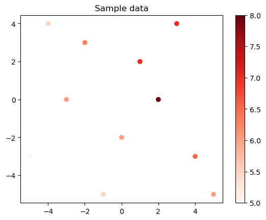
For the needs of this guide, the following sample data has been created:

import numpy as np

m = np.array([-5, -4, -3, -2, -1, 0, 1, 2, 3, 4, 5])
n = np.array([-3, 4, 0, 3, -5, -2, 2, 0, 4, -3, -5])

X = np.column_stack([m, n])
y = np.array([5, 5.5, 6, 6.3, 5.5, 6, 7, 8, 7, 6.5, 6])

Now, the data can be loaded for further processing.

kgn.load(X, y)

Note that the X variable is simply a 2D numpy array in which the first column stores longitude values & the second column stores latitude values. The y variable is a vector that matches the length of the longitude/latitude column.

The GeoKrige package handles also Multidimensional Kriging, so more dimensions can be included in the X variable. For more information about Multidimensional Kriging, please refer to this section.

Variogram - The Foundation of Any Kriging Method

Although various Kriging Methods may yield slightly different predictions, they all rely on the same fundamental principles. The unknown values are estimated on the basis of a function fitted to a created variogram. The function fitted to the variogram quantifies the dissimilarity between a pair of points, and this is a fundament to determine weight that the point with a measured value will have in the process of estimating unknown value in another point.

In Kriging, the variogram is a plot that allows to visualize the dissimilarity between points with measured values as a function of distance. The variogram can be easily created with the GeoKrige package as follows:

kgn.variogram(bins=10)

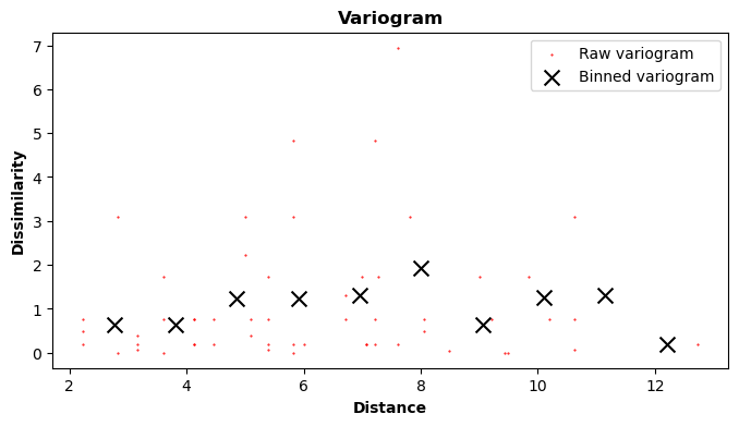
The variogram method automatically plots the variogram. The number of bins specified in the bins parameter is crucial and has a significant impact on the interpolation results. There is no universal rule that will dictate how many bins should be created. Simply put, the bins parameter specifies into how many bins the points with measured values will be binned. Then, a single bin dissimilarity is an average dissimilarity of all points inside that specific bin.

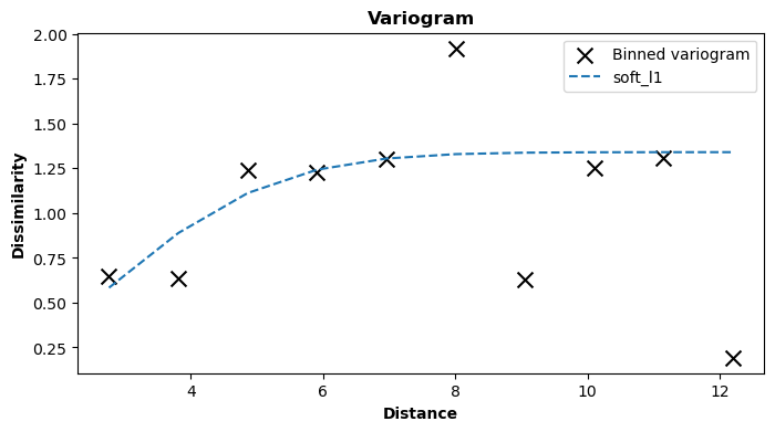
Now that it is clear how dissimilarity corresponds to the distance between points, the variogram function can be fitted. The parameters can be fitted automatically, but they can also be fixed manually by the user. In this tutorial, the parameters will be estimated automatically. For more information about fixing parameters manually, please see this section of the documentation.

By default, there are four variogram models to select:

• gaussian
• exp (exponential)
• linear
• spherical

Users can define their own variogram models, but this will not be covered in this tutorial. The variogram model can be changed with the model parameter. By default, there is the gaussian variogram model.

kgn.fit()

At this moment, the Kriging Model is ready to make predictions. However, there is one more component worth having a look at – a covariance matrix. The covariance matrix shows how a specific pair of points with measured values is correlated with each other.

kgn.plot_cov_matrix()

The covariance between points with measured values is calculated on the basis of a covariance function that uses the parameters estimated in the process of fitting the variogram function. The variogram and covariance functions are two fundamental components of every variogram model. For more information about variogram model functions, please refer to this section of the documentation.

Note that the kgn.summarize() method plots all of the above plots on the same figure, so it may be handy in some cases.

Using the Kriging Model to make predictions

To utilize the created Kriging Model for predictions, it is essential to first generate an appropriate mesh grid. A mesh grid consists of densely spaced points arranged in a rectangular grid, generated based on two vectors (or more for multidimensional mesh grids). These vectors undergo a Cartesian Product to form the grid, with separate matrices storing values for each coordinate axis.

In a 2D mesh grid, two matrices are generated: one for x-coordinates and the other for y-coordinates. Both matrices have the same shape, allowing specific coordinates in space to be extracted using their indices. For instance, if a point represented by indices [1, 2] in matrix A (x-coordinates) is considered, the second component in a pair can be found at the same position in matrix B (y-coordinates).

A mesh grid can be easily generated with the meshgrid function from the numpy package. In the case below, the meshgrid function will return two matrices clipped together in a list – the first element in the list will correspond to the x-coordinates matrix, and the second element in the list will correspond to the y-coordinates matrix (A & B matrices from the image above).

import numpy as np

lon = np.linspace(-6, 6, 10)
lat = np.linspace(-6, 6, 10)
meshgrid = np.meshgrid(lon, lat)

The predict method of the trained Kriging Model accepts mesh grids as input, so the meshgrid variable can be passed to the method. Predictions are then calculated for the points stored in the mesh grid & another matrix with the same shape as the mesh grid matrices is returned.

Z = kgn.predict(meshgrid)

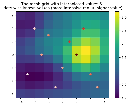
The Z variable is a matrix with the same shape as matrices in the meshgrid variable, so this fact can be used to effortlessly plot the interpolation results with the matplotlib package.

import matplotlib.pyplot as plt

X, Y = meshgrid
plt.pcolormesh(X, Y, Z)  # contour/countrf methods are also good here

plt.colorbar()
plt.scatter(m, n, c=y, cmap='Reds')  # the generated sample data
plt.title('The mesh grid with interpolated values & \n dots with known values (more intensive red -> higher value)')

plt.show()

The predict method is designed to accept mesh grids created with the numpy.meshgrid function and return another mesh grid with interpolated results. It can also receive as an input 2D matrices of the numpy.ndarray objects, and in this case a vector of the same length as the 2D matrix is returned. When there is a need of predicting values for single points (not for a mesh grid), then 2D matrix of numpy.ndarray type should be passed as an argument.

In fact, the numpy.meshgrid function returns a list with nested numpy.ndarray objects inside (matrices). So, when the predict method receives as an input a list, it assumes that a mesh grid has been passed. Because of this, a list that imitates 2D matrix passed as an input will raise an error.

Additionally, the GeoKrige package handles GeoDataFrame & rasterio objects very well, and it can transform both to a mesh grid that is ready to be passed as an argument to the predict method. The classes handling mentioned objects have also other useful features such as masking created mesh grids to polygons of a GeoDataFrame object. For more information, please visit these tutorials: Using GeoKrige with GeoPandas, Using GeoKrige with rasterio.

The Kriging Model evaluation

The GeoKrige package supports a simple evaluation of the final results with the evaluate method. The method uses a cross-validation approach and returns MAE (Mean Absolute Error) & RMSE (Root-Mean-Square Error).

kgn.evaluate(seed=3)

>>> Mean Absolute Error: 0.7039604146571146
>>> Root-Mean-Square Error: 0.7780971156412542

The seed parameter specifies a seed for the numpy.random module. Setting the parameter to a specific value ensures that identical results will be produced in each evaluation rerun. When the seed value is set to None, the cross-validation groups are created randomly, resulting in potentially different evaluation results across runs.

In the scenario described in this tutorial, with a MAE totaling around 0.70, it implies that the predicted values may deviate from the actual values by approximately ±0.70 on average.

However, determining whether this level of accuracy is satisfactory depends on various factors, such as the specific application, the acceptable margin of error, and the consequences of inaccurate predictions. As there is no universal interpretation rule for MAE, the assessment of the model's performance should consider the context and requirements of the problem at hand.

The Start Guide Wrap Up

1. kgn.load()
2. kgn.variogram()
3. kgn.fit()
4. kgn.predict()
5. kgn.evaluate()